Project · In progress since June 2026
Solar Modelling Web App
A physics-based model of how much energy a solar installation produces anywhere on Earth, hour by hour, built to design two-axis sun-tracking systems.
What it is
My honours thesis asked what limits the performance of solar panels that track the sun on two axes. This project turns that question into a tool. You drop a pin anywhere on a map, and the model simulates all 8,760 hours of a typical year at that spot using real weather records. It reports what a tracking system would produce against a conventional fixed-tilt array, and how much is lost to heat, dust, snow, shading and ageing.
The aim has narrowed as the work went on. Rather than one tool that does everything, it is one validated core from which precise single-purpose instruments can be cut: a site comparison, a battery sizing check, a shading study. That only works if every equation in the core is documented and checked, which is why so much of this page is about method.
A sample simulation
These numbers came from the model on 16 November 2026, with default module settings and no obstructions. Two sites: Perth, where I live, and Munich, for contrast.
Figure 1
Two sites, one model
| Perth, Australia | Munich, Germany | |
|---|---|---|
| Two-axis tracking yield | 615 kWh/m² | 358 kWh/m² |
| Fixed-tilt reference yield | 424 kWh/m² | 263 kWh/m² |
| Tracking gain | +45% | +36% |
| Optimal fixed tilt | 27° | 42° |
| Yield exceeded 9 years in 10 (P90) | 601 kWh/m² | 340 kWh/m² |
| Year-to-year variability | 1.7% | 4.0% |
| Heat loss | 4.4% | 3.6% |
| Snow loss, no clearing | none | 6.5% |
| Dust loss, no cleaning | 0.2% | 0.2% |
| Climate-adjusted degradation | 0.68% per year | 0.38% per year |
| Output after 25 years | 83% | 89% |
The contrast is the point. Perth produces about 70% more energy per square metre, and its output barely varies from year to year. Munich loses more than 6% to snow if nobody clears the panels, while Perth loses more to heat. Hot sites also age panels faster: the model's climate-adjusted degradation rate is nearly double in Perth, so after 25 years a Perth panel has lost more of its output than a Munich one.
Figure 2
Perth, month by month
View as a table
| Month | Two-axis | Fixed tilt |
|---|---|---|
| Jan | 70.9 | 41.8 |
| Feb | 58.4 | 39.0 |
| Mar | 53.2 | 38.5 |
| Apr | 48.1 | 35.1 |
| May | 39.1 | 30.5 |
| Jun | 35.1 | 26.7 |
| Jul | 31.9 | 24.8 |
| Aug | 41.5 | 32.0 |
| Sep | 45.0 | 33.4 |
| Oct | 58.6 | 39.7 |
| Nov | 64.0 | 40.2 |
| Dec | 69.1 | 42.0 |
How the model is built
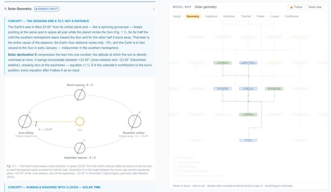
The core is a chain of physical models, each feeding the next: where the sun is, how much light arrives, how much lands on the panel, how hot the cell runs, what power comes out, and what is lost along the way. Each link is documented with its equation, its source in the literature, and the exact code that implements it.
The models, in the order the energy flows:
- Sun position and irradiance. Solar geometry for every hour, with measured beam, diffuse and ground-reflected light from the European PVGIS dataset.
- Tracking and fixed-tilt incidence. Light on a panel that follows the sun, and on a fixed panel at its best tilt, with reflection losses at shallow angles.
- Cell temperature. A wind-aware thermal model, because a breezy site runs panels more than ten degrees cooler than the industry's still-air assumption.
- Electrical output. A single-diode model of the module, read from a real datasheet, including bifacial panels that collect light on both faces.
- Losses. Dust build-up and rain cleaning, snow cover and shedding, far and near shading, and 25 years of climate-dependent degradation.
- Confidence. Year-to-year variability from four decades of weather, so a result is a range rather than a single hopeful number.
- Storage. Battery behaviour, wiring, conversion losses and the temperature inside the enclosure.
The documentation is part of the product. Every section of the model is explained inside the app to a teaching standard: a plain-language concept, a figure drawn from scratch, the real equations with a hover definition on every symbol, a worked example and a table of where each value comes from. If a user cannot follow how a number was produced, the number is not finished. The whole section is published as its own page, linked below, with the interactive map of the model beside the text.
Figure 3
The methodology section and model map
Where it is heading
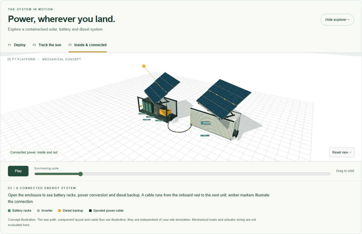
The model underpins a hardware idea: a solar, battery and backup generator system packed into a shipping container, with a two-axis tracking array that folds out on arrival. The app's landing page carries an interactive concept of it.
Figure 4
The container concept
How the project is run
I direct this project and an AI system does most of the building. That arrangement only works with structure, and the structure has become as much a part of the project as the physics.
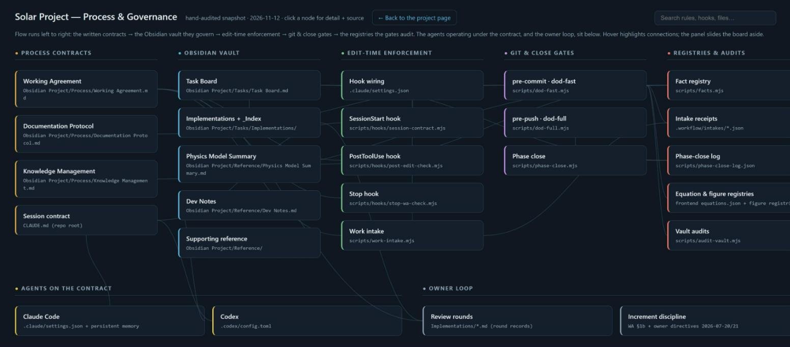
- A notes vault as the single source of truth. Goals become tasks, tasks drive code, and code is recorded back as an as-built document, all in the same change. Each topic has exactly one owning document.
- A written working agreement. A standing contract the AI reads at the start of every session: check primary sources before stating a fact, list everything a change affects before making it, challenge a flawed instruction rather than comply, and report outcomes faithfully.
- Automatic checks. Scripts run after every edit, before every save to the project history and before every publish. They compare documented facts against the code, test the interface in a real browser, and block the change if anything disagrees.
- Small reviewed increments. Work arrives in pieces I can audit, each with a short guide to what I should see and where the rough edges are.
- The ratchet. Any rule that gets broken twice stops being a rule and becomes an automatic check.
Figure 5
The project in numbers
| Changes committed since June 2026 | more than 630 |
| Busiest months | July (267) and August (305) |
| Hours simulated per site | 8,760 |
| Blocks on the model map | 34 |
| Subsystems that open into their own equations | 20 |
| Weather record behind the variability estimate | 39 years |
The full governance structure is drawn as an interactive map, with excerpts from the actual rules and checks.
Figure 6
The process and governance map
Read more
Three essays use this project as their worked example: Terminology, Methodology, Technology on how the domain was mapped, Incentive Structures and Feedback Loops on why the rules are shaped as they are, and Co-Directing with AI on how the work is verified.